Mandelbrot.

(to be elaborated in future).

See, if You wish: Mandelbrot Set on Wikipedia.


Image.




Java Code.

import java.awt.Color;
import java.io.File;
import java.awt.image.BufferedImage;
import javax.imageio.ImageIO;

public class PaintMandelbrot {
    public static void main(String[] args) throws Exception {
        int width = 1920, height = 1080, max = 1000;
        BufferedImage image = new BufferedImage(width, height, BufferedImage.TYPE_INT_RGB);
        int black = 0;
    int[] colors = new int[max];
    for (int i = 0; i<t;max; i++) {
            colors[i] = Color.HSBtoRGB(i/128f+3/4f, 1, i/(i+8f));
        }

        for (int row = 0; row < height; row++) {
            for (int col = 0; col < width; col++) {
                double c_re = (col - width/2)*4.0/width;
                double c_im = (row - height/2)*4.0/width;
                double x = 0, y = 0;
                double r2;
                int iteration = 0;
                while (x*x+y*y < 4 && iteration < max) {
                    double x_new = x*x-y*y+c_re;
                    y = 2*x*y+c_im;
                    x = x_new;
                    iteration++;
                }
                if (iteration < max) image.setRGB(col, row, colors[iteration]);
                else image.setRGB(col, row, black);
            }
        }

        ImageIO.write(image, "png", new File("d:\\mandelbrot.png"));
    }
}

Fermat's Little Theorem.

Introduction.

Prime Numbers have uses in Cryptography, important part of Computer Sciences.

Functional Paradigm uses Mathematics for Computing extensively, therefore this article.


Fermat's Little Theorem.

If p is a prime number and a is a natural number, then:

a^p≡a (mod p).

Furthermore, if p does not divide a, then there exists some smallest exponent d such that:

a^d-1≡0 (mod p)

and d divides p-1. Hence,

a^(p-1)-1≡0 (mod p).

The theorem is sometimes also simply known as 'Fermat's theorem' (Hardy and Wright 1979, p. 63).

This is a generalization of the Chinese hypothesis and a special case of Euler's totient theorem. It is sometimes called Fermat's primality test and is a necessary but not sufficient test for primality. Although it was presumably proved (but suppressed) by Fermat, the first proof was published by Euler in 1749. It is unclear when the term 'Fermat's little theorem' was first used to describe the theorem, but it was used in a German textbook by Hensel (1913) and appears in Mac Lane (1940) and Kaplansky (1945).

The theorem is easily proved using mathematical induction on a. Suppose p|a^p-a (i.e., p divides a^p-a). Then examine:

(a+1)^p-(a+1).

From the binomial theorem,



Rewriting,



But p divides the right side, so it also divides the left side. Combining with the induction hypothesis gives that p divides the sum:



as assumed, so the hypothesis is true for any a. The theorem is sometimes called Fermat's simple theorem. Wilson's theorem follows as a corollary of Fermat's little theorem.

Fermat's little theorem shows that, if p is prime, there does not exist a base a < p with (a,p)=1 such that a^(p-1)-1 possesses a nonzero residue modulo p. If such base a exists, p is therefore guaranteed to be composite. However, the lack of a nonzero residue in Fermat's little theorem does not guarantee that p is prime. The property of unambiguously certifying composite numbers while passing some primes make Fermat's little theorem a compositeness test which is sometimes called the Fermat compositeness test. A number satisfying Fermat's little theorem for some nontrivial base and which is not known to be composite is called a probable prime.

Composite numbers known as Fermat pseudoprimes (or sometimes simply 'pseudoprimes') have zero residue for some as and so are not identified as composite. Worse still, there exist numbers known as Carmichael numbers (the smallest of which is 561) which give zero residue for any choice of the base a relatively prime to p. However, Fermat's little theorem converse provides a criterion for certifying the primality of a number. A table of the smallest pseudoprimes P for the first 100 bases a follows (OEIS A007535; Beiler 1966, p. 42 with typos corrected).

2	341	22	69	42	205	62	63	82	91
3	91	23	33	43	77	63	341	83	105
4	15	24	25	44	45	64	65	84	85
5	124	25	28	45	76	65	112	85	129
6	35	26	27	46	133	66	91	86	87
7	25	27	65	47	65	67	85	87	91
8	9	28	45	48	49	68	69	88	91
9	28	29	35	49	66	69	85	89	99
10	33	30	49	50	51	70	169	90	91
11	15	31	49	51	65	71	105	91	115
12	65	32	33	52	85	72	85	92	93
13	21	33	85	53	65	73	111	93	301
14	15	34	35	54	55	74	75	94	95
15	341	35	51	55	63	75	91	95	141
16	51	36	91	56	57	76	77	96	133
17	45	37	45	57	65	77	247	97	105
18	25	38	39	58	133	78	341	98	99
19	45	39	95	59	87	79	91	99	145
20	21	40	91	60	341	80	81	100	153
21	55	41	105	61	91	81	85

Source: Wolfram MathWorld.

Congruence.

Introduction.

Prime Numbers have uses in Cryptography, important part of Computer Sciences.

Functional Paradigm uses Mathematics for Computing extensively, therefore this article.


Congruence.

If two numbers b and c have the property that their difference b-c is integrally divisible by a number m (i.e., (b-c)/m is an integer), then b and c are said to be 'congruent modulo m.' The number m is called the modulus, and the statement 'b is congruent to c (modulo m)' is written mathematically as:





If b-c is not integrally divisible by m, then it is said that 'b is not congruent to c (modulo m),' which is written:



The explicit '(mod m)' is sometimes omitted when the modulus m is understood by context, so in such cases, care must be taken not to confuse the symbol ≡ with the equivalence sign.

The quantity b is sometimes called the 'base,' and the quantity c is called the residue or remainder. There are several types of residues. The common residue defined to be nonnegative and smaller than m, while the minimal residue is c or c-m, whichever is smaller in absolute value.



Congruence arithmetic is perhaps most familiar as a generalization of the arithmetic of the clock. Since there are 60 minutes in an hour, 'minute arithmetic' uses a modulus of m=60. If one starts at 40 minutes past the hour and then waits another 35 minutes, 40+35≡15 (mod 60), so the current time would be 15 minutes past the (next) hour.



Similarly, 'hour arithmetic' on a 12-hour clock uses a modulus of m=12, so 10 o'clock (a.m.) plus five hours gives 10+5≡3 (mod 12), or 3 o'clock (p.m.)

Congruences satisfy a number of important properties, and are extremely useful in many areas of number theory. Using congruences, simple divisibility tests to check whether a given number is divisible by another number can sometimes be derived. For example, if the sum of a number's digits is divisible by 3 (9), then the original number is divisible by 3 (9).

Congruences also have their limitations. For example, if a≡b and c≡d (mod n), then it follows that a^x≡b^x, but usually not that x^c≡x^d or a^c≡b^d. In addition, by 'rolling over,' congruences discard absolute information. For example, knowing the number of minutes past the hour is useful, but knowing the hour the minutes are past is often more useful still.

Let a≡a^' (mod m) and b≡b^' (mod m), then important properties of congruences include the following, where => means 'implies':

1. Equivalence: a≡b (mod 0)=>a≡b (which can be regarded as a definition).

2. Determination: either or .

3. Reflexivity: a≡a (mod m).

4. Symmetry: a≡b (mod m) => b≡a (mod m).

5. Transitivity: a≡b (mod m) and b≡c (mod m) => a≡c (mod m).

6. a+b≡a^'+b^' (mod m).

7. a-b≡a^'-b^' (mod m).

8. ab≡a^'b^' (mod m).

9. a≡b (mod m) => ka≡kb (mod m).

10. a≡b (mod m) => aⁿ≡bⁿ (mod m).

11. a≡b (mod m₁) and a≡b (mod m₂) => a ≡b (mod [m₁,m₂]), where [m₁,m₂] is the least common multiple.

12. , where (k,m) is the greatest common divisor.

13. If a≡b (mod m), then P(a)≡P(b) (mod m), for P(x) a polynomial.

Properties (6-8) can be proved simply by defining:

a=a^'+rm
b=b^'+sm,

where r and s are integers. Then:

a+b=a^'+b^'+(r+s)m
a-b=a^'-b^'+(r-s)m
ab=a^'b^'+(a^'s+b^'r+rsm)m,

so the properties are true.

Congruences also apply to fractions. For example, note that:

2×4≡1 3×3≡2 6×6≡1 (mod 7),

so:

1/2≡4 1/4≡2 2/3≡3 1/6≡6 (mod 7).

To find p/q (mod m) where (q,m)=1 (i.e., q and m are relatively prime), use an algorithm similar to the greedy algorithm. Let q₀≡q and find:



where is the ceiling function, then compute:

q₁≡q₀p₀ (mod m).

Iterate until q_n=1, then:



This method always works for m prime, and sometimes even for m composite. However, for a composite m, the method can fail by reaching 0 (Conway and Guy 1996).

Finding a fractional congruence is equivalent to solving a corresponding linear congruence equation:

ax≡b (mod m).

A fractional congruence of a unit fraction is known as a modular inverse.

Source: Wolfram MathWorld.

Predicate Logic Basics.

Introduction.

This article joins the 'functional programming paradigm' with 'programming in logic', an another important & very well known programming paradigm.

We'll be using both a little of the 'Sets Theory', as well as 'Mathematical Analysis' & 'Logic'.


Predicates.

In mathematics, a predicate is commonly understood to be a Boolean-valued function P: X → {true, false}, called the predicate on X.


Predicate Language Syntax.

Logical formulas of the 'Predicate Calculus' are built from symbols, set of these symbols is called 'alphabet'.

To fully specify 'alphabet' we would need to include all of the symbols that belong to it.

For simplicity, we'll provide a definition that will specify only types of symbols, that might be included in 'alphabet'.


def. 1. A 'predicate calculus alphabet' consists of following symbols:
- constants,
- variables,
- function symbols,
- predicate symbols,
- logical functors,
- parentheses.


def. 2. For a given 'predicate calculus alphabet' the 'terms set' is defined as follows:
- each of constants is a 'term',
- each of variables is a 'term',
- if 'f' is a 'm-argument function symbol' and t₁, t₂, ... , t_m are terms,
    then f(t₁, t₂, ... , t_m) is a 'term'.


The 'terms' in the 'predicate calculus' are arguments of the 'predicate symbols'.

Predicate symbols assign each of the 'term argument' a boolean value from a set of {true, false}.

Assigning a 'predicate symbol' to a 'term argument' gives in a result the simplest of 'logical formulas', called also: 'atomic formula'.


def. 3. For each m-argument 'predicate symbol': 'R', if t₁, t₂, ... , t_m are 'terms',
    then R(t₁, t₂, ... , t_m) is an 'atomic formula'.


The 'complex formulas' are created by joining 'atomic formulas' using 'logical functors' and parentheses. Possibilities of creating 'complex formulas' are specified by the following definition.

def. 4. For a given 'alphabet', the 'predicate calculus formulas set' is defined as follows:
- each of the 'atomic formula' is a 'formula',
- for any 'formula' α, the (α) and ¬α are 'formulas',
- for any 'formulas' α and β, the α∧β, α∨β, α→β, α↔β are 'formulas',
- for any 'formula' α with a variable v, there are 'formulas': (∀_v)α and (∃_v)α.


Predicate Language Semantics.

Semantics for a 'predicate calculus' are defined by specifying a 'model', in which 'formulas' are interpreted.


def. 5. A 'model' is a pair <X, ι>, where X is a non-empty set called a 'domain' and ι is 'interpretation function' which:
- assigns for each of constants a certain 'domain' element,
- assigns for each of 'm-argument function symbol' a certain mapping from X^m on X,
- assigns for each of 'm-argument predicate symbol' a certain mapping from X^m on {true, false}.


In this context, predicates are treated as the 'relation names', for whose an 'interpretation function' assigns the 'relations on domain'.


def. 6. A 'valuation' of variables for a domain X is any function with a domain containing all of variables, with values in a set X.


For a given model and variables valuation, formulas can be valuated to specify their 'boolean value'.

We'll give only a definition for 'atomic formulas', for the 'complex formulas' can be specified using the known interpretation of the 'logical functors'.


def. 7. For a model <X,ι> and a variable valuation v, the values of the terms are specified as follows:
- for any constant x: V^v_{X, ι}(v) = ι(x);
- for any variable v: V^v_{X, ι}(v) = v(v);
- for any m-argument function symbol f and any terms t₁, ... , t_m:
     V^v_{X, ι}(f(t₁, ... , t_m)) = ι(v)(V^v_{X, ι}(t₁), ... , V^v_{X, ι}(t_m)).

Let's notice that a value of ι(v) is a function, with a value in a 'functions space', as defined in def. 5.

Then we interpret ι(v)(V^v_{X, ι}(t₁), ... , V^v_{X, ι}(t_m)) as a complex function composition.


def. 8. For a model <X,ι> and a variable valuation v,
    the value of an 'atomic formula' R(t₁, ... , t_m), where:
      R is an m-argument predicate symbol,
      t₁, t₂, ... , t_m are terms,
        is specified as follows:
          V^v_{X, ι}(R(t₁, ... , t_m)) = ι(R)(V^v_{X, ι}(t₁), ... , V^v_{X, ι}(t_m)).

Again a value of ι(v) is a function, we have a complex function composition here as well.


Formulas' logical value are basis to specify: satisfiedness, satisfiability & truthfulness of the boolean formulas.


def. 9. Any formula α is satisfied in a model with a variable valuation v, when:
    V^v_{X, ι}(α) = 'true'.

def. 10. Any formula α is satisfiable, if there exists a model and a variable valuation, for which α is satisfied.

def. 11. Any formula α is true, when for any model and a variable valuation:
    α is satisfied.


Symetrically we define falsifiedness, falisfiability & falseness of the boolean formulas.

The 'falseness' property can also be defined using formulas' sets.

def. 12. Formulas set F_S is false (self-contradictory), when conjunction of all formulas from this set F_S is not satisfiable.


Entailment & Inference in a Predicate Calculus.

There are two types of consequences, as far as the 'entailment & inference in a predicate calculus' reaches:
- semantic consequence (logical consequence, entailment),
- syntactic consequence (inference).


def. 13. Formula α is a semantic consequence of a formulas set { β₁, β₂, ... , β_m }, if for all models and variable valuations, for which formula β₁ ∧ β₂ ∧ ... ∧ β_m is satisfied, formula α is also satisfied. We can note it as: { β₁, β₂, ... , β_m } ⊧ α.


Syntactic consequence is defined, by assuming a certain inference system, consisting of a logical axioms set & of a inference rules set. Axioms are logical formulas, rules specify a way of deriving formulas from different formulas.


An inference rule noted as follows:



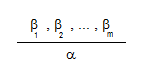
Means that based on formulas: β₁, β₂, ... , β_m (that are premises), we can infer in a single step the formula α (that is a conclusion).


def. 14. A proof of a formula α based on a formulas set S is:
    a serie of formulas:
      β₁, β₂, ... , β_m = α,
        in which for every i = 1, 2, ..., m :
          a formula β_i is:
            - an axiom,
            - or a S-set element,
            - or a result of using a certain inference rule on rules preceding it in a proof.


deft. 15. A formula α is a syntactic consequence of a formulas set S, in a certain inference system, if in this a system exists a proof of this formula based on S. We can note it as: S ⊦ α.


def. 16. Inference system is correct, if for any formulas set S and an α formula, a syntactic consequence S ⊦ α entails semantic consequence S ⊧ α.


def. 17. Inference system is complete, if for any formulas set S and an α formula, a semantic consequence S ⊧ α entails syntactic consequence S ⊦ α.


There are many different (assuming different axioms & inference rules) correct & complete inference systems for the predicate calculus.