Sunday, 17 November 2013

Prime Numbers.

Prime Number.

A 'Prime Number' is a natural number greater than 1 that has no proper divisors other than 1 and itself.

The Natural Numbers are 0, 1, 2, 3, 4, ....

The list of prime numbers starts with 2, 3, 5, 7, 11, 13, .... Except for 2, all of these are odd, of course.


Haskell Implementation for Prime Number Test.

1. Let's define divides function.

It should check if number m divides n, and this is true when and only when remainder of dividing n by m equals 0. The definition of divides function can therefore be phrased in terms of a predefined function rem for finding the remainder of a division process:


divides m n = ((rem n m) == 0)


in Haskell, symbol '=' is used for "is defined as" and symbol '==' for identity relation (and operator). Single apostrophes are used in this phrase only for showing terminal symbols boundaries. Terminal symbol is single "word" in "programming language", from which no other "words" can be produced, so it's not a "definition" or "production". For more details, please read Literature about languages and compilers.

A line of Haskell code of the form: foo t = .... (or: foo t1 t2 = .... , or: foo t1 t2 t3 = .... , and so on) is called a Haskell equation. In such an equation, foo is called the function and t its formal argument (or: t1 t2 t3 its formal arguments).

Thus, in the Haskell equation: divides m n = ((rem n m) == 0) , divides is the function, m is the first formal argument, and n is the second formal argument.


2. Let's test 'divides' function.

We can put definition of divides in a file: 'prime.hs'. After that we can start Haskell Interpreter and load that file in memory.

Prelude> :l prime

Then we can call it, to execute as follows:

*Main>divides 5 7

or

*Main>divides 5 30

When executed, it will be parsed, or converted into processor instructions and will return results 'immediately', without prior compilation needed. Because it's interpreted by Interpreter, instead of being compiled by Compiler.
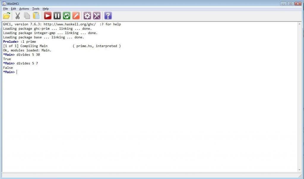
Divides function execution in Haskell. photo divides_haskell_zps5a2e7cb0.jpg


3. Let's define & test 'ld' function.

'ld' stands for 'least divisor'.

For convenience we can define supporting function 'ldf' that finds least divisor (pl: 'dzielnik') of a dividend (pl: 'dzielna') n, starting from a given threshold (pl: 'próg') k, with k ≤ n.

This means we are to find least divisor of n, which is not less than k.


We have:


ld n = ldf 2 n

ldf k n | divides k n = k
          | k^2 > n = n
          | otherwise = ldf (k+1) n


(TODO: explain, nicely and precisely, what happens in above example, and how we can think about guarded equations, such as with 'ldf' function.)

(TODO: finish Haskell Implementation for Prime Number Test).

(Source: [1]).

Saturday, 16 November 2013

Fern.


Barnsley's Fern.

for source code or image files click on a corresponding image in a Fractal gallery to the left side of this blog.


Barnsley's Fern.

The fern is one of the basic examples of self-similar sets, i.e. it is a mathematically generated pattern that can be reproducible at any magnification or reduction. Like the Sierpinski triangle, the Barnsley fern shows how graphically beautiful structures can be built from repetitive uses of mathematical formulas with computers.

Barnsley's book about fractals is based on the course which he taught for undergraduate and graduate students in the School of Mathematics, Georgia Institute of Technology, called Fractal Geometry. After publishing the book, a second course was developed, called Fractal Measure Theory. Barnsley's work has been a source of inspiration to graphic artists attempting to imitate nature with mathematical models.

The fern code developed by Barnsley is an example of an iterated function system (IFS) to create a fractal. He has used fractals to model a diverse range of phenomena in science and technology, but most specifically plant structures.

"IFSs provide models for certain plants, leaves, and ferns, by virtue of the self-similarity which often occurs in branching structures in nature. But nature also exhibits randomness and variation from one level to the next; no two ferns are exactly alike, and the branching fronds become leaves at a smaller scale. V-variable fractals allow for such randomness and variability across scales, while at the same time admitting a continuous dependence on parameters which facilitates geometrical modelling. These factors allow us to make the hybrid biological models..."

—Michael Barnsley.


Paint Tutorial.

Though Barnsley's fern could in theory be plotted by hand with a pen and graph paper, the number of iterations necessary runs into the tens of thousands, which makes use of a computer practically mandatory. Many different computer models of Barnsley's fern are popular with contemporary mathematicians. As long as the math is programmed correctly using Barnsley's matrix of constants, the same fern shape will be produced.

The first point is painted at the origin (x0 = 0, y0 = 0) and then the new points are painted as described by functions f1, f2, f3 and f4, each resulting from Bernsley's matrix of constants transformations. Which function to use in given iteration, is determined 'randomly', as based on probablity factor from Bernsley's matrix of constants.

f1:

xn+1 = 0
yn+1 = 0.16*yn

This coordinate transformation is chosen 1% of the time and just maps any point to a point in the first line segment at the base of the stem. This part of the figure is the first to be completed in during the course of iterations.

f2:

xn+1 = 0.85*xn + 0.04*yn
yn+1 = −0.04*xn + 0.85*yn+1.6

This coordinate transformation is chosen 85% of the time and maps any points inside the leaflets.

f3:

xn+1 = 0.2*xn − 0.26*yn
yn+1 = 0.23*xn + 0.22*yn + 1.6

This coordinate transformation is chosen 7% of the time and maps point inside the leaflet (or pinna) to a point across the stem (one side).

f4:

xn+1 = −0.15*xn + 0.28*yn
yn+1 = 0.26*xn + 0.24*yn + 0.44

This coordinate transformation is chosen 7% of the time and maps point inside the leaflet (or pinna) to a point across the stem (other side).

The first coordinate transformation draws the stem. The second generates successive copies of the stem and bottom fronds to make the complete fern. The third draws the bottom frond on the left. The fourth draws the bottom frond on the right. The recursive nature of the IFS guarantees that the whole is a larger replica of each frond. Note that the complete fern is within the range −2.1820 < x < 2.6558 and 0 ≤ y < 9.9983.

(Source).

Critic is requested and welcome.

Fractals.

def. 'Fractal is a figure or surface generated by successive subdivisions of a simpler polygon or polyhedron, according to some iterative process'.

(Source).